User defined S-N curve and Basquin Expression
- Chetan G.
01/2021
Symbols
- $S_u$ = Ultimate tensile strength
- $S_a$ = Stress Amplitude
- $k$ = Constant exponent
- $N$ = Fatigue life
- $\sigma'_f$ = Fatigue Strength Coefficient
- $b$ = Fatigue Strength Exponent
- $\Delta \sigma_1$ = maximum principal stress
- $\frac{\Delta \sigma_1} {2}$ = maximum principal stress amplitude
- $N_f$ = Number of cycles
- $2N_f$ = Number of reversal to failure
- $\sigma_m$ = mean stress along the principal axis
When using NX Simcenter Durability Specialist module fatigue material properties should be assigned. For "Stress Life" approach, the user should either:
- define the S-N curve as a table or
- Fatigue Strength Coefficient ($ \sigma'_f $) and Fatigue Strength Exponent ($ b $) values should be entered as stress life expression.
The purpose of this document is to illustrate the fatigue strength expressions.
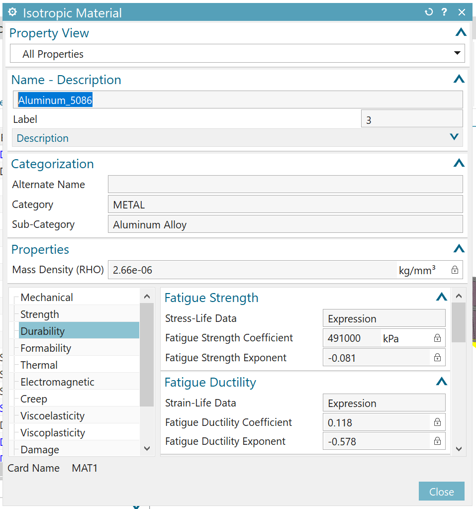
Often for a large range of fatigue life (N) the relation between $log S_a$ and $log N$ is approximately linear. This gives us the following relation:
$ S_a^k * N = constant $ ..[textbook formulation, Schijve, 2001]
$ \frac{\Delta \sigma_1}{2} = \sigma'_f (2N_f)^b$ ..[Siemens formulation, withouth mean stress effect]
$ \frac{\Delta \sigma_1}{2} = (1-\frac{\sigma_m}{S_u}) \sigma'_f (2N_f)^b$ ..[Siemens formulation, Goodman method for mean stress effect]
Now, let us plot the S-N curve based on the fatigue strength expression given in the figure above.
$\sigma'_f = 491$ [MPa]
$b = -0.081$
%matplotlib inline
import numpy as np
import matplotlib.pyplot as plt

def basquin_plot(sigma_coeff, b_expo):
    x_axis = np.geomspace(1, 10000000, num=8)
    y_axis = sigma_coeff* np.power(x_axis, b_expo)
    plt.xlabel('Cycles (N)')
    plt.ylabel('Stress amlpitude (S_a)')
    plt.yscale('log')
    plt.xscale('log')
    plt.plot(x_axis, y_axis)
    plt.grid(which='both')
basquin_plot(sigma_coeff=491, b_expo=-0.081)
Note that in the above plot, y-axis is stress amplitude, which is $\frac{\Delta \sigma_1}{2}$. If user defined S-N curve values are determined by experiments, make sure to enter the correct values.
Next, let us illustrate the calculation of number of cycles (life) based on the applied stresses. Following codes implements the basquin expression in terms of number of cycles for given stress and in terms of applied stress given the number of cycles. (Without mean stress effect.)
def basquin(sigma_coeff, b_expo, delta_sigma):
    #sigma_coeff and sigma_delta have the same units ex: [MPa]
    cycles = 0.5*np.power(10, (np.log10((delta_sigma/2) / sigma_coeff) / b_expo))
    print('life='+str(cycles))
    return cycles

def basquin_rev(sigma_coeff, b_expo, cycles):
    # sigma_coeff and sigma_delta have the same units ex: [MPa]
    delta_sigma = 2*sigma_coeff* np.power(2*cycles, b_expo)
    print('delta_sigma='+str(delta_sigma))
    return delta_sigma
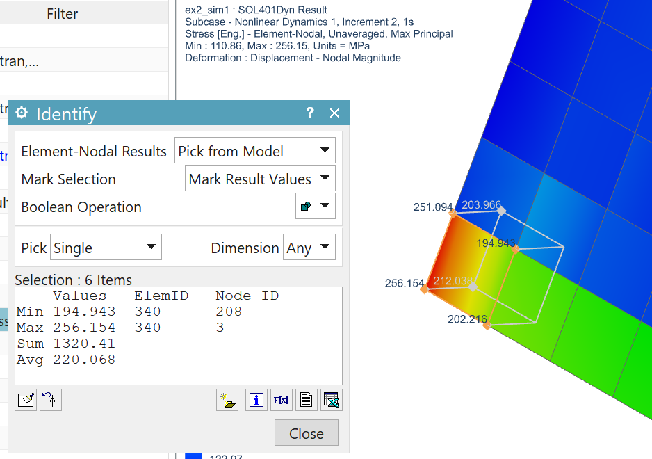
Let us consider the results of a small exercise of dynamic analysis using SOL401 in NX.
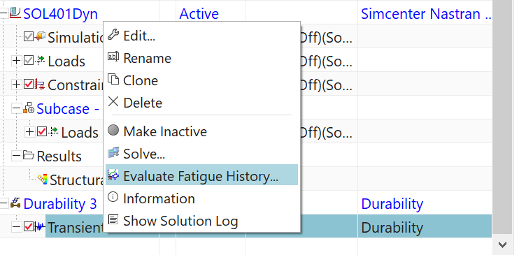
Next, the stress fatigue history is evaluted using the Durability Specialist of NX Simcenter as shown in the figure above. The result of element 340 is shown below:
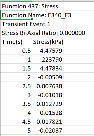
Note, that the maximum principal stress evaluated by the Nastran solver SOL401 is used in the evaluation of fatigue stress history by the Durability specialist. Durability solver uses its own stress axis method. (Question: how does this method work?)
Finally, the durability is solved. The life for element ID 340 is shown in the figure below:
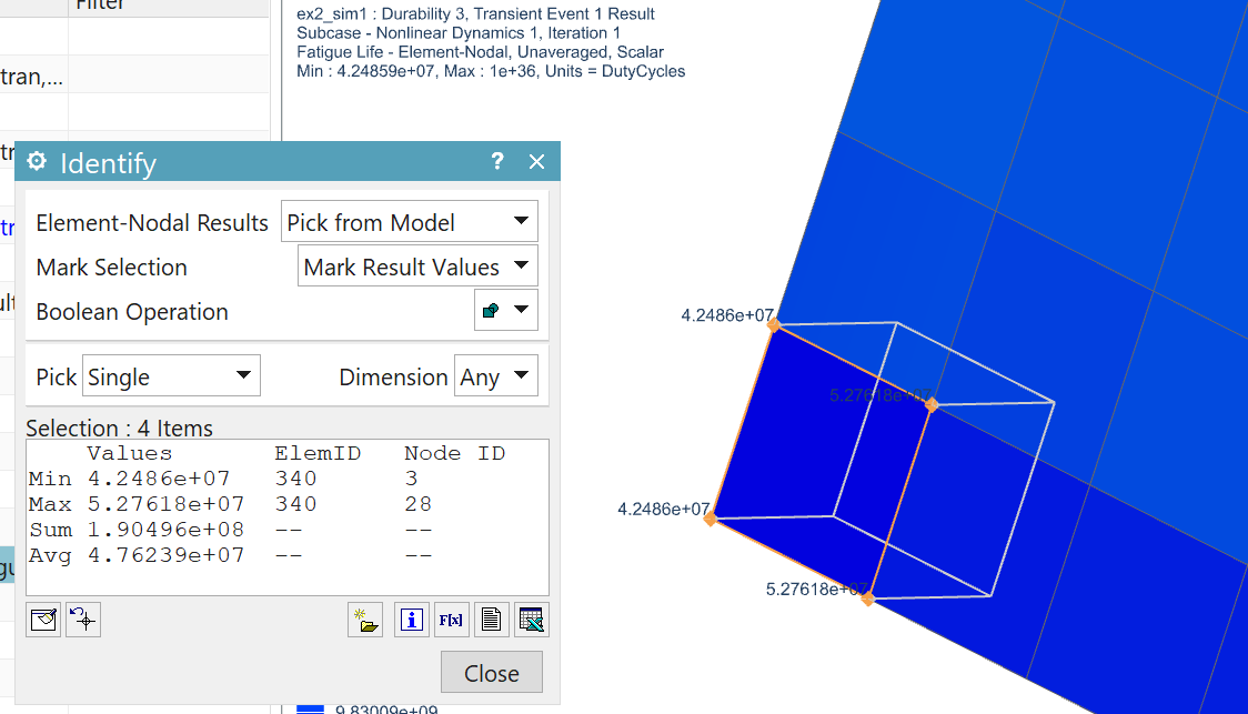
We can now cross check the results, by solving the basquin expressions.
life = basquin(delta_sigma=223.79, sigma_coeff=491, b_expo=-0.081)
sigma_delta=basquin_rev(cycles=4.2486e+07, sigma_coeff=491, b_expo=-0.081)
Note that due to logarithmic nature of the S-N curve, small increase in stress can result is large decrease in the expected life. For, example if we had used maximum principal stress of 256.15[Mpa] as the input for fatigue evaluation, then resulting life would be five times low.
life = basquin(delta_sigma=256.15, sigma_coeff=491, b_expo=-0.081)
References:
- Schijve, J. (2001). Fatigue of structures and materials. Springer Science & Business Media.
- Stress Life - Siemens documentation
https://docs.plm.automation.siemens.com/tdoc/nx/1899/nx_help#uid:xid1128419:index_advanced:xid385327:id635096:id624881:id975729 - Siemens documentation pages
https://docs.plm.automation.siemens.com/tdoc/nx/1899/nx_help#uid:xid1128419:index_advanced:xid1593960
https://docs.plm.automation.siemens.com/tdoc/nx/1899/nx_help#uid:xid1128419:index_advanced:xid385327
https://docs.plm.automation.siemens.com/tdoc/nx/1899/nx_help#uid:xid1128419:index_advanced:xid385327:id973964
https://docs.plm.automation.siemens.com/tdoc/nx/1899/nx_help#uid:xid1128419:index_advanced:xid1593960:xid1604043:xid1604038:xid1604027
https://docs.plm.automation.siemens.com/tdoc/nx/1899/nx_help#uid:xid1128419:index_advanced:xid385327:id635096:id624881:xid456177